Demo 3: Solving Boundary Integral Equations (BIEs)

The code (tutorial/demo3-bie-solve.cpp) demonstrates how to solve boundary integral equations (BIEs) using the CSBQ library. In this demo we solve the Stokes Dirichlet boundary value problem (BVP) around a circular ring.

Step 1: Problem Definition

Given a bounded domain \(\Omega \in \mathbb{R}^3\) with boundary \(\Gamma = \partial\Omega\), we want to solve the Stokes Dirichlet boundary value problem in the exterior of the domain,

\[\begin{split}\Delta \mathbf{u} - \nabla p &= 0 \quad \mbox{ in } \mathbb{R}^3 \setminus \overline{\Omega}, \\ \nabla \cdot \mathbf{u} &= 0 \quad \mbox{ in } \mathbb{R}^3 \setminus \overline{\Omega}, \\ \mathbf{u}|_{\Gamma} &= \mathbf{u}_0 \quad \mbox{ on } \Gamma.\end{split}\]

where \(\mathbf{u}\) and \(p\) are the unknown fluid velocity and pressure in \(\mathbb{R}^ \setminus \overline{\Omega}\), and \(\mathbf{u}_0\) is the given fluid velocity on \(\Gamma\). In addition, we also assume that the fluid velocity at infinity decays to zero,

\[\mathbf{u}(\mathbf{x}) \rightarrow \mathbf{0} \quad \mbox{ as } |\mathbf{x}| \rightarrow \infty.\]

Step 2: Integral Equation Formulation

In the exterior of \(\Omega\), we represent the fluid velocity using the combined field representation,

\[\mathbf{u} = \mathcal{D}[\mathbf{\sigma}] + \eta \, \mathcal{S}[\mathbf{\sigma}] \quad \mbox{ in } \mathbb{R}^3 \setminus \overline{\Omega},\]

where \(\eta\) is a scaling factor, \(\mathcal{S}\) and \(\mathcal{D}\) are the Stokes single-layer and double-layer potential operators,

\[\begin{split}\mathcal{S}[\mathbf{\sigma}](\mathbf{x}) &\colon= \int_{\Gamma} S(\mathbf{x} - \mathbf{y}) \, \mathbf{\sigma}(\mathbf{y}) \, dS_{\mathbf{y}}, \\ \mathcal{D}[\mathbf{\sigma}](\mathbf{x}) &\colon= \int_{\Gamma} D(\mathbf{x} - \mathbf{y}) \, \mathbf{\sigma}(\mathbf{y}) \, dS_{\mathbf{y}}, \\\end{split}\]

and \(\mathbf{\sigma}\) is an unknown density on \(\Gamma\). With this representation, \(\mathbf{u}\) satisfies the Stokes equations in the exterior domain and the velocity decay condition at infinity. Applying the boundary condition on \(\Gamma\), we get a second-kind boundary integral equation (BIE) formulation,

\[(I/2 + D + \eta \, S) \mathbf{\sigma} = \mathbf{u}_0 \quad \mbox{ on } \Gamma,\]

where \(S\) and \(D\) are the Stokes single-layer and double-layer boundary integral operators. After discretizing and solving for the unknown \(\sigma\), we can evaluate the velocity field \(\mathbf{u}\) anywhere in \(\mathbb{R}^3 \setminus \overline{\Omega}\) using the combined field representation formula above.

Step 3: Discretize the Geometry

We create an object of type SlenderElemList and load the geometry file data/ring.geom into this object:

SlenderElemList<double> elem_lst;
elem_lst.Read<double>("data/ring.geom", comm);

This is a collective MPI operation and the geometry is partitioned between the participating MPI processes in the communicator comm. Refer to demo-1 to see how to build a geometry discretization.

Step 4: Discretize and Solve the Integral Equation

• Define a Custom Kernel:

  We build a custom kernel function that evaluates the sum of the Stokes double-layer kernel and the scaled single-layer kernel. The scaling parameter is passed as a template parameter.

  template <Long SL_scal> struct Stokes3D_CF_ {
    static const std::string& Name() {
      // Name determines what quadrature tables to use.
      // Single-layer quadrature tables also works for combined fields.
      static const std::string name = "Stokes3D-FxU";
      return name;
    }
  
    static constexpr Integer FLOPS() {
      return 50;
    }
  
    template <class Real> static constexpr Real uKerScaleFactor() {
      return 1 / (8 * const_pi<Real>());
    }
  
    template <Integer digits, class VecType>
    static void uKerMatrix(VecType (&u)[3][3], const VecType (&r)[3], const VecType (&n)[3], const void* ctx_ptr) {
      using Real = typename VecType::ScalarType;
      const auto SL_scal_ = VecType((Real)SL_scal);
      const auto r2 = r[0]*r[0] + r[1]*r[1] + r[2]*r[2];
      const auto rinv = approx_rsqrt<digits>(r2, r2 > VecType::Zero()); // Compute inverse square root
      const auto rinv2 = rinv * rinv;
      const auto rinv3 = rinv2 * rinv;
      const auto rinv5 = rinv3 * rinv2;
      const auto rdotn = r[0] * n[0] + r[1] * n[1] + r[2] * n[2];
      const auto rdotn_rinv5_6 = VecType((Real)6) * rdotn * rinv5;
      for (Integer i = 0; i < 3; i++) {
        for (Integer j = 0; j < 3; j++) {
          const auto ri_rj = r[i] * r[j];
          const auto ker_dl = ri_rj * rdotn_rinv5_6; // Double-layer kernel
          const auto ker_sl = (i == j ? rinv + ri_rj * rinv3 : ri_rj * rinv3); // Single-layer kernel
          u[i][j] = ker_dl + ker_sl * SL_scal_; // Combine kernels
        }
      }
    }
  };
  using Stokes3D_CF = GenericKernel<Stokes3D_CF_<4>>;
  

  For more details see defining custom kernels in SCTL.

• Initializing the Layer Potential Operator:

  Next, we create a layer-potential operator using our custom kernel. We set the accuracy, and add the element list to the operator.

  Stokes3D_CF ker;
  BoundaryIntegralOp<double, Stokes3D_CF> LayerPotenOp(ker);
  LayerPotenOp.SetAccuracy(tol);
  LayerPotenOp.AddElemList(elem_lst);
  

• Defining the Boundary Integral Operator:

  Define the boundary integral operator using a lambda function:

  const auto BIO = [&LayerPotenOp](Vector<double>* U, const Vector<double>& sigma) {
    LayerPotenOp.ComputePotential(*U, sigma);
    (*U) += sigma * 0.5;
  };
  

• Solving the Boundary Integral Equation:

  We solve the boundary integral equation for the unknown sigma using the GMRES solver. We define the boundary condition, set up the GMRES solver, and solve the system.

  Vector<double> sigma, U0(LayerPotenOp.Dim(0));
  U0 = 1; // Set boundary condition to (Ux, Uy, Uz) = (1, 1, 1)
  GMRES<double> solver(comm);
  solver(&sigma, BIO, U0, tol);
  

Step 5: Post-processing

After solving the BIE, evaluate the velocity field in the volume and visualize it.

CubeVolumeVis<double> cube(50, 2.0, comm); // 50x50x50 points, side length 2
LayerPotenOp.SetTargetCoord(cube.GetCoord()); // Set target coordinates for the operator
Vector<double> U;
LayerPotenOp.ComputePotential(U, sigma);
cube.WriteVTK("vis/bie-solution", U - 1); // Write to VTK file

A cubic volume with 50x50x50 points and a side length of 2 is defined using the CubeVolumeVis class. We then evaluate the boundary integral operator at the discretization nodes to get the fluid velocity field, and write the VTK visualization of the fluid velocity field to the file vis/bie-solution.pvtu.

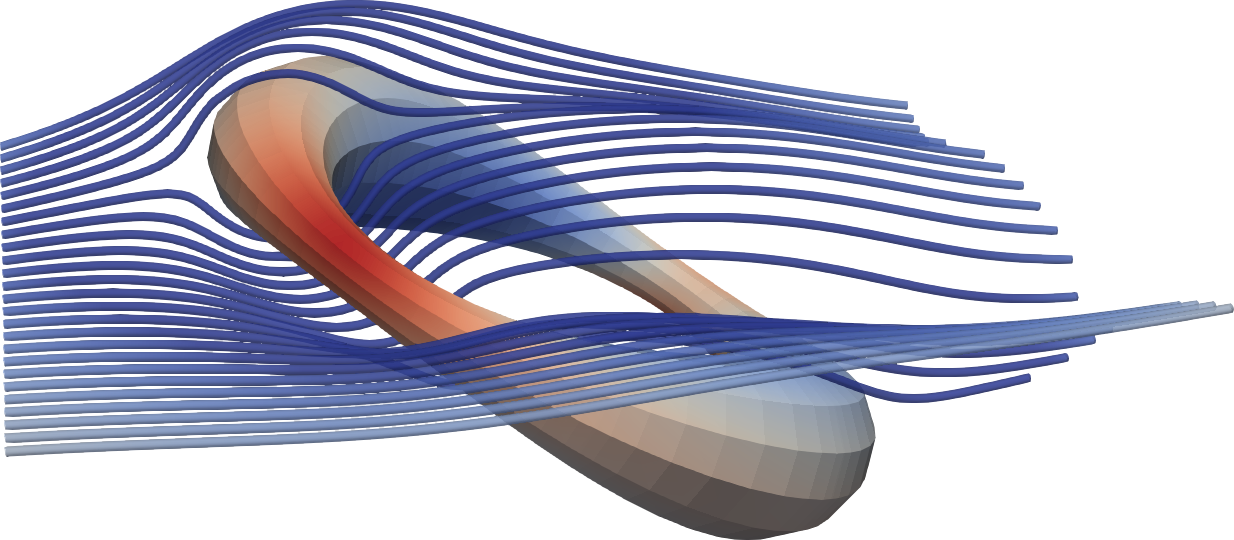
Streamlines visualizing Stokes flow around a circular ring.

Compiling and Running the Code

• Without MPI: Navigate to the project root directory and run:

  make bin/demo3-bie-solve && ./bin/demo3-bie-solve
  

• With MPI: In the project root directory, edit Makefile to set CXX=mpicxx and uncomment CXXFLAGS += -DSCTL_HAVE_MPI. Then, run:

  make bin/demo3-bie-solve && mpirun -n 2 --map-by slot:pe=1 ./bin/demo3-bie-solve
  

This will solve a Stokes Dirichlet BVP in the exterior of a loop geometry and write the solution density sigma to a VTK visualization file vis/sigma.pvtu. It will also write a VTK visualization of the fluid velocity field in the volume to the file vis/bie-solution.pvtu.

Complete Example Code

/**
 * This demo code shows how to solve BIEs (boundary integral equations). In
 * particular, we show how to:
 *
 * 1) Define a custom kernel type.
 *
 * 2) Build a BIO (boundary integral operator) with a custom kernel.
 *
 * 3) Solve a boundary integral equation using the BIO and GMRES.
 *
 * 4) Visualize the computed potentials.
 *
 * To compile and run the code, start in the project root directory and run:
 * make bin/demo3-bie-solve && ./bin/demo3-bie-solve
 */

#include <csbq.hpp>
using namespace sctl;

// Define a custom kernel for Stokes combined field (double-layer + scaled single-layer potential)
template <Long SL_scal> struct Stokes3D_CF_ {
  // Function to return the name of the kernel
  static const std::string& Name() {
    // Name determines what quadrature tables to use.
    // Single-layer quadrature tables also works for combined fields.
    // Not compatible with PVFMM, since it is not scale invariant
    // (single- and double-layer kernels have different scales)
    static const std::string name = "Stokes3D-FxU";
    return name;
  }

  // Function to return the number of floating point operations
  static constexpr Integer FLOPS() {
    return 50;
  }

  // Function to return the scale factor for the kernel
  template <class Real> static constexpr Real uKerScaleFactor() {
    return 1 / (8 * const_pi<Real>());
  }

  // Function to compute the kernel matrix
  template <Integer digits, class VecType>
  static void uKerMatrix(VecType (&u)[3][3], const VecType (&r)[3], const VecType (&n)[3], const void* ctx_ptr) {
    using Real = typename VecType::ScalarType;
    const auto SL_scal_ = VecType((Real)SL_scal);
    const auto r2 = r[0]*r[0] + r[1]*r[1] + r[2]*r[2]; // Compute squared distance
    const auto rinv = approx_rsqrt<digits>(r2, r2 > VecType::Zero()); // Compute inverse square root
    const auto rinv2 = rinv * rinv;
    const auto rinv3 = rinv2 * rinv;
    const auto rinv5 = rinv3 * rinv2;
    const auto rdotn = r[0] * n[0] + r[1] * n[1] + r[2] * n[2];
    const auto rdotn_rinv5_6 = VecType((Real)6) * rdotn * rinv5;
    for (Integer i = 0; i < 3; i++) {
      for (Integer j = 0; j < 3; j++) {
        const auto ri_rj = r[i] * r[j];
        const auto ker_dl = ri_rj * rdotn_rinv5_6; // Double-layer kernel
        const auto ker_sl = (i == j ? rinv + ri_rj * rinv3 : ri_rj * rinv3); // Single-layer kernel
        u[i][j] = ker_dl + ker_sl * SL_scal_; // Combine kernels
      }
    }
  }
};

// Define a type alias for the custom kernel
using Stokes3D_CF = GenericKernel<Stokes3D_CF_<4>>;

int main(int argc, char** argv) {
  Comm::MPI_Init(&argc, &argv);

  {
    const Comm comm = Comm::World();
    double tol = 1e-8; // Tolerance for accuracy

    SlenderElemList<double> elem_lst;
    elem_lst.Read<double>("data/ring.geom", comm); // read geometry data from file
    SCTL_ASSERT_MSG(elem_lst.Size() > 0, "Could not read geometry file.");

    Stokes3D_CF ker;
    BoundaryIntegralOp<double,Stokes3D_CF> LayerPotenOp(ker, false, comm); // Create the layer-potential
    LayerPotenOp.SetAccuracy(tol);                                         // Set the accuracy tolerance
    LayerPotenOp.AddElemList(elem_lst);                                    // Add the element list to the operator

    // Define the boundary-integral operator: (I/2 + D + S * scale_factor)
    const auto BIO = [&LayerPotenOp](Vector<double>* U, const Vector<double>& sigma) {
      LayerPotenOp.ComputePotential(*U, sigma);
      (*U) += sigma * 0.5;
    };

    Vector<double> sigma, U0(LayerPotenOp.Dim(0)); // Vectors for sigma (density), and U0 (boundary condition)
    U0 = 1;                                        // Set boundary condition to (Ux, Uy, Uz) = (1, 1, 1)
    GMRES<double> solver(comm);                    // Define GMRES solver
    solver(&sigma, BIO, U0, tol);                  // Solve the linear system
    elem_lst.WriteVTK("vis/sigma", sigma, comm);   // Write sigma to VTK file

    // Visualize the fluid velocity in the volume
    CubeVolumeVis<double> cube(50, 2.0, comm);   // Define a cubic volume with 50x50x50 points and side length 2
    LayerPotenOp.SetTargetCoord(cube.GetCoord());// Set target coordinates for the operator
    Vector<double> U;                            // Vector for storing the velocity field
    LayerPotenOp.ComputePotential(U, sigma);     // Evaluate the velocity field
    cube.WriteVTK("vis/bie-solution", U - 1);    // Write to a VTK file
  }

  Comm::MPI_Finalize();
  return 0;
}